 SpanDraft
Analytical reference cases
This chapter belongs to the detailed evidence of the Solver verification. It compares all cases for which the validation catalog contains a closed-form solution with the SpanDraft calculation.
Derivation of the references
The references begin with equilibrium of the overall system. From it follow the support reactions and the moment curve . The deflection curve arises by integrating the beam equation twice, with the constants of integration from the boundary conditions.1
The calculation runs with exact rational numbers and calls SpanDraft nowhere. Only for storing are the results converted to floating-point numbers. The reference is thus independent of the solver but deliberately rests on the same beam theory. It checks the solution of the model and not the model.
The formulas below state the loads , and as magnitudes; their direction is given in the respective caption. All results follow the SpanDraft sign convention: is positive upward, and a sagging moment is positive. Cases V01 to V06 use . In the figures, moments are given in Nm and deflections in m. The curves are scaled to their largest magnitude in each figure.
What is compared per case
The table at the end of the chapter lists 87 or 63 individual comparisons per case. Case V01 is composed as follows:
| Comparison | Scope | Number |
|---|---|---|
| Fields | 12 evaluation points with , , , , and each | 72 |
| Support reactions | and at the pinned support, at the roller support | 3 |
| Extreme values | minimum and maximum of , and | 6 |
| Extreme locations | location and side of these six extreme values | 6 |
Evaluation points lie at the beam ends, at supports, at load locations and at the boundaries of distributed loads; at interior locations of this kind, left and right are separate. Additional evaluation points are placed at the relative positions and, in each subinterval between two such locations, the points at 37 % and 63 %. The fields are thus also checked between the nodes.
Simply supported and cantilever
V01: central point force
At the load location, the moment has a kink and the shear force a jump.
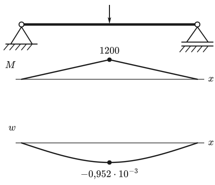
Analytical
at
SpanDraft
at
V02: cantilever with end force
The fixed support provides a force reaction and a moment reaction.
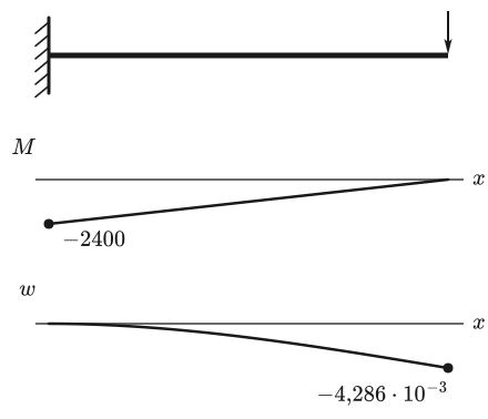
Analytical
at
SpanDraft
at
V03: cantilever under distributed load
The moment is quadratic, the deflection curve a polynomial of fourth degree.
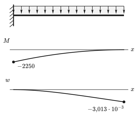
Analytical
at
SpanDraft
at
V04: simply supported under distributed load
There is no station at midspan. Both extreme values therefore lie in the interior of a piece.
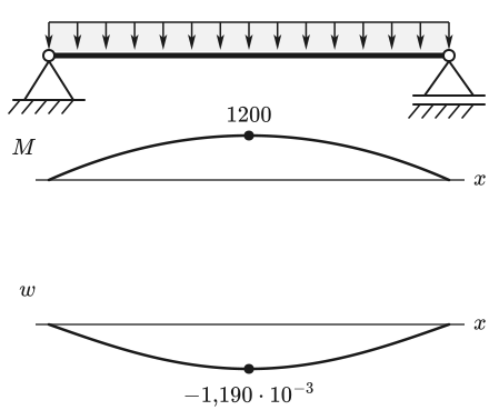
Analytical
at
SpanDraft
at
Jumps and extreme values next to the load location
V05: interior point moment
The moment jumps by at the load location. The deflection curve remains continuous and smooth and lies above the initial position over the entire length.
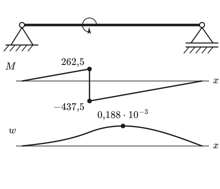
Analytical
at from
SpanDraft
at
V06: asymmetric point force
The largest sag does not lie under the load, and there is no station at its location.
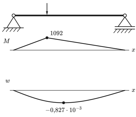
Analytical
at for
SpanDraft
at
Fields between the stations
Extreme values alone do not show whether the field between the stations is correct. V06 has only three event stations: the two supports and the load location. The values in between come from the analytical curves of the pieces. Four of the evaluation points in the comparison:
| in m | in mm, analytical | in mm, SpanDraft | in Nm, analytical | in Nm, SpanDraft |
|---|---|---|---|---|
| 0.548 | −0.388837 | −0.388837 | 498.68 | 498.68 |
| 1.332 | −0.768186 | −0.768186 | 1040.52 | 1040.52 |
| 2.472 | −0.722743 | −0.722743 | 595.92 | 595.92 |
| 3.492 | −0.281101 | −0.281101 | 198.12 | 198.12 |
Other orders of magnitude
The three variants of V04 check the same system at very different lengths, loads and stiffnesses. They are complete cases with both programs and all physical checks. The formulas from V04 apply unchanged. V04-S01 and V04-S03 show the same digits of the deflection because grows by exactly the factor between them.
| Case | in m | in N/m | in Nm² | in Nm, analytical | in Nm, SpanDraft | in m, analytical | in m, SpanDraft |
|---|---|---|---|---|---|---|---|
| V04-S01 | 0.1 | 6 | 168 | 0.0075 | 0.0075 | ||
| V04-S02 | 1 | 60 | 5600 | 7.5 | 7.5 | ||
| V04-S03 | 10 | 600 | 7500 | 7500 |
How close the values are
The comparisons are rounded to six digits and therefore show equal digits. The actual check works with the unrounded values and the tolerance condition from the short version. The measure is the utilization of this tolerance. For , the tolerance would be exactly exhausted.
The table gives the largest utilization over all compared values for each case. Extreme locations are not included, because there it is checked whether the SpanDraft location belongs to the set of reference locations.
| Case | Individual comparisons | Largest utilization | Status |
|---|---|---|---|
| V01 | 87 | passed | |
| V02 | 63 | passed | |
| V03 | 63 | passed | |
| V04 | 63 | passed | |
| V05 | 87 | passed | |
| V06 | 87 | passed | |
| V04-S01 | 63 | passed | |
| V04-S02 | 63 | passed | |
| V04-S03 | 63 | passed | |
| Total | 639 | passed |
The utilization is calculated with the current solver against the same stored references as in the acceptance. For the other nine cases, no analytical reference is stored, although they too are in principle analytically solvable. They are checked by the chapter External reference solvers.
Sources
- Felix Udoeyo. Deflection of Beams: Geometric Methods. Structural Analysis, Section 7.3 Deflection by Method of Double Integration, Temple University Press / North Broad Press. 2020. Accessed .