 SpanDraft
External reference solvers
This chapter belongs to the detailed evidence of the Solver verification. It describes the check against two independent programs, also for the systems for which the validation catalog contains no analytical reference.
Cases without an analytical reference
For cases V01 to V06 and the three variants of V04, the validation catalog contains an independently derived closed-form solution; they are given in the chapter Analytical reference cases. The nine cases V07 to V15 are, as linear beam problems, in principle also analytically solvable, but the catalog stores no independent analytical reference provider for them. Their references are therefore solely the two programs, complemented by the physical and metamorphic checks.
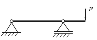
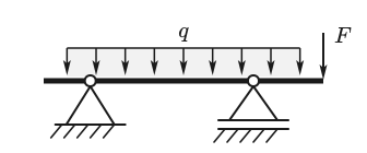
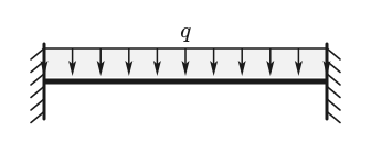
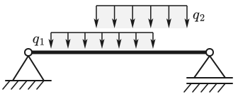
Beams with two supports
These cases check overhangs, fixed supports at both ends and the superposition of distributed loads.
Continuous beams
With more than two supports, each span depends on its neighbors. The cases check individually loaded spans, loads above interior supports, and forces and moments at load boundaries.
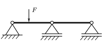
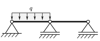
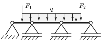
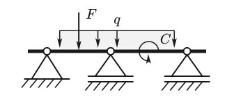
The fifth continuous beam, V14 with the force exactly above the interior support, is covered in the section Non-applicable comparisons.
Two programs with different strengths
The two programs complement each other, and both arrive at the result by a different solution path than SpanDraft: IndeterminateBeam integrates the deflection curve symbolically, PyCBA sets up a stiffness method from beam elements. Neither uses the state formulation of SpanDraft.
| Property | IndeterminateBeam | PyCBA |
|---|---|---|
| Version | 2.4.01 | 1.0.22 |
| Author | Jesse Bonanno3 | Colin Caprani4 |
| Solution path | symbolic integration of , equilibrium and compatibility at the supports5 | direct stiffness method: global matrix from the spans, boundary conditions, nodal displacements, then reactions and internal forces and moments6 |
| Beam theory in this check | : The shear part of the deformation is omitted. | not set: exact Euler–Bernoulli element6 |
| Fields between the nodes | polynomial sections generated by the program | grid per element, cubically interpolated; at nodes the degrees of freedom themselves |
| Available quantities | , , , , , , , | , , , , , |
Quantities that a program does not supply are not replaced by assumed zero values. They are missing from the comparisons of this program. For IndeterminateBeam, is determined by differentiating the expression for generated by the program.
Discrepancies are not resolved by majority vote. They are investigated systematically, starting with the model and supports, followed by theory, units, load definition, signs, side conventions and numerical tolerance, until the cause is found.
Both programs are pure check tools in fixed versions, run with CPython 3.9.6. They belong neither to the delivered application nor to its build, and nothing of their code is adopted into SpanDraft.
Sign alignment
SpanDraft calculates with to the right, upward and counterclockwise. Forces upward and moments counterclockwise are positive, means tension, a sagging moment, and holds. The derivation of this convention is given in the mechanical fundamentals.
Inputs and results are converted only when the programs are interfaced. The actual comparison logic knows no program-dependent sign rules.
| Quantity | IndeterminateBeam | PyCBA |
|---|---|---|
| Input point force, distributed load | unchanged | negated, because load magnitudes there are positive downward |
| Input point moment | unchanged | unchanged |
| Reactions , | unchanged | unchanged |
| , , , | unchanged | unchanged |
| , | unchanged | not available |
| not available | not available |
This conversion is not merely assumed. Both programs were calculated against the closed-form solution directly on all nine analytical cases, without SpanDraft: 18 pairings with 909 individual comparisons, all passed. A sign or unit error in the interface would have been noticed there.
Jump locations and extreme values
At a jump location, a field has different values on the left and on the right. Both are compared separately, without averaging and without evaluation at . For IndeterminateBeam, the polynomial section of the respective open interval is continued up to the exact boundary point. For PyCBA, the sides come from the separate results of the adjoining elements.
An extreme value can occur at several locations or over an entire section. The references therefore store the complete set of locations, and SpanDraft names one representative. It is checked whether this one belongs to the set. In V01, the largest shear force is reached over the entire section from 0 to 2 m, and SpanDraft names .
The plateau includes its inner boundary value. The opposite side of a force jump, in contrast, is not accepted as equivalent: a dedicated test ensures that the comparison fails in this case.
Tolerances
Each individual comparison must satisfy the tolerance condition. The limits were not changed in the course of the acceptance, not even in investigating deviations.
| Quantity | absTol | relTol |
|---|---|---|
| Force, reaction, , | ||
| Moment, reaction moment | ||
| , | ||
| Extreme location |
For the tolerance utilization, the same definition applies as in the chapter Analytical reference cases. Figure 9 shows it for all cases and references, calculated with the current solver against the stored references. For PyCBA, the largest values occur for and , which between the nodes come from an interpolated grid. The largest value overall is at V15. For V14, SpanDraft deviates from PyCBA by exactly zero, which is why the point is missing there.

Grid convergence of PyCBA
PyCBA outputs the fields between the nodes on a grid. A result between the grid points is thus itself an approximation. It may serve as a reference only if a refinement no longer changes it appreciably.
The check therefore begins with 1024 subdivisions per element and doubles them up to at most 131 072. All values, extreme locations and plateau boundaries must change by at most 0.1 of their comparison tolerance over two consecutive doublings, and the structure of the location sets must remain stable. In addition, the drift of the grid values at the element ends relative to the nodal degrees of freedom must not exceed the same limit. All 18 cases converge.
Figure 10 shows the curve for V04. Here the drift decides: only 32 768 and 65 536 pass as two consecutive refinements. The observed convergence order is 2.
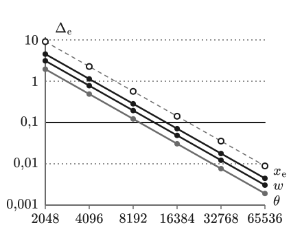
The stored references contain the curve of every refinement. A pass without this convergence evidence is rejected. The final grids are given in the table under Comparison counts per case.
Non-applicable comparisons
Exactly six individual comparisons are documented as not applicable: the extreme locations , , , , and of case V14 against IndeterminateBeam.
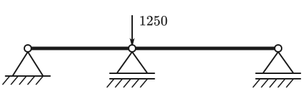
The force acts exactly at a support in its constrained direction. Physically, at the interior support, all other reactions and all fields are zero. For a zero field, every location takes the same extreme value; there is no unique extreme location. IndeterminateBeam delivers tiny rounding residues here instead of zero, and their extreme locations say nothing about the physical zero field.
The classification is narrowly limited. All six extreme values remain mandatory comparisons and passed, as did the 60 field values and four reactions of this case. PyCBA is fully applicable for V14, including the six location comparisons. The exception is tied to this case, its input and this program version. Non-applicable comparisons are counted separately and not scored as passed.
Deep dive: the residual fields of IndeterminateBeam in V14
On the intervals from 0 to 2.5 m and from 2.5 to 6 m, the program delivers two non-constant cubic residual polynomials for and two non-constant linear residual polynomials for . For , there are two different constants of and . The reason lies in solving with floating-point numbers inside the program.
In the stored values, the residues are at most , , and . The raw locations remain unchanged in the reference file. Setting the residues to zero or merging the shear force plateaus would be an additional assumption that the program does not support. This was therefore not done.
Deep dive: findings during the acceptance
Two further deviations occurred during the acceptance. Both lay in the evaluation of the reference programs and not in SpanDraft. Tolerances were not changed for them.
- V12 against PyCBA: Differentiating the interpolated deflection curve produced an additional, artificial stationary point near the fixed support, so that the location set did not converge. The extremum search has since used the field supplied by the program. The case converges at 65 536 subdivisions.
- V13 against both programs: When redundant plateau boundaries were removed, a permissible side was lost. The location agreed, and there is no force jump at this distributed load boundary. Now only sides in the interior of a plateau are removed.
Comparison counts per case
The number of individual comparisons grows with the number of evaluation points and supports. The table gives the values of the acceptance runs of October 3, 2026 and November 11, 2026, which agree.
| Case | IndeterminateBeam | PyCBA | Not applicable | Final grid PyCBA | Status |
|---|---|---|---|---|---|
| V01 | 75 | 62 | 0 | 32768 | passed |
| V02 | 55 | 46 | 0 | 16384 | passed |
| V03 | 55 | 46 | 0 | 16384 | passed |
| V04 | 55 | 46 | 0 | 65536 | passed |
| V05 | 75 | 62 | 0 | 16384 | passed |
| V06 | 75 | 62 | 0 | 16384 | passed |
| V07 | 75 | 62 | 0 | 32768 | passed |
| V08 | 135 | 110 | 0 | 32768 | passed |
| V09 | 96 | 79 | 0 | 16384 | passed |
| V10 | 76 | 63 | 0 | 32768 | passed |
| V11 | 157 | 128 | 0 | 65536 | passed |
| V12 | 58 | 48 | 0 | 65536 | passed |
| V13 | 135 | 110 | 0 | 8192 | passed |
| V14 | 70 | 63 | 6 | 4096 | passed |
| V15 | 196 | 159 | 0 | 8192 | passed |
| V04-S01 | 55 | 46 | 0 | 16384 | passed |
| V04-S02 | 55 | 46 | 0 | 32768 | passed |
| V04-S03 | 55 | 46 | 0 | 131072 | passed |
| Total | 1553 | 1284 | 6 | passed |
Reproducibility
The 18 case inputs exist as neutral files and feed SpanDraft and all references. The results of the references are stored in 45 files: 36 from the two programs and 9 analytical. Each file names the program version, runtime environment, sign rules and the checksums of input and calculation scripts. A changed input invalidates the associated reference, and outdated files make the check fail.
A complete recalculation reproduced all 45 files exactly except for the time of generation. The normal check run compares against these stored files and needs neither Python nor the two programs. References are replaced only by an explicit, reviewed step and never automatically.
Sources
- Jesse Bonanno. indeterminatebeam 2.4.0. Python Package Index. 2025. Accessed .
- Colin Caprani. PyCBA 1.0.2. Python Package Index. 2026. Accessed .
- Jesse Bonanno. IndeterminateBeam: A Python package for solving 1D indeterminate beams. Journal of Open Source Education 4 (40), 111. 2021. DOI 10.21105/jose.00111. Accessed .
- Colin Caprani. PyCBA: Python Continuous Beam Analysis. Software documentation. Accessed .
- Jesse Bonanno. Theory. IndeterminateBeam, software documentation. Accessed .
- Colin Caprani. pycba.analysis.BeamAnalysis. PyCBA, software documentation. Accessed .