 SpanDraft
Cross-section geometry and properties
Cross-section and beam model
The cross-section enters the beam model with three different quantities that do not replace one another:
- The area describes how much material is present. Together with the density, it determines the optional self-weight. SpanDraft does not need the axial stiffness , because there are no axial loads.
- The second moment of area describes how this area is distributed about the selected bending axis. Together with Young’s modulus, it yields the flexural rigidity and thus determines the deformation.
- The section modulus relates to the distance of the outermost fiber. It does not influence the deformation but links the calculated bending moment with the elastic edge stress.1
That alone does not determine the flexural rigidity is already shown by a rectangle of 20 mm × 60 mm: standing on edge, it has nine times the second moment of area of the flat position for identical area. The following sections describe how SpanDraft determines these quantities from the geometry.
From outline to area and centroid
The geometry lies in a local plane: points horizontally to the right, vertically upward. It consists of an outer contour and optional inner contours that describe cutouts. Each contour is a closed sequence of straight lines and exact circular arcs.
Area and centroid coordinates are defined by area integrals1:
The centroid is a result of the geometry. It does not have to lie within the material, as the example in Figure 1 shows.
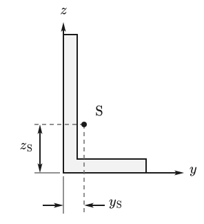
For these integrals, SpanDraft does not divide the area into elements. With Green’s theorem, they can be converted into contour integrals around the boundary, so that the segments of the contour suffice. For a straight segment between the points and , the area contribution is
This is the signed triangle area between the reference point and the segment. The sum over the closed contour yields the enclosed area. From the same segment endpoints, SpanDraft also determines the first and second moments of area analytically.
Circular arcs are not approximated by polygons. An arc is composed of the contribution of its chord and the analytical circular segment between chord and arc. The chord is treated like a straight segment. For the circular segment with radius and opening angle , the following holds, for example,
Depending on the direction in which the arc is traversed, this contribution is added or subtracted. The first and second moments of area of the circular segment also enter the sum analytically.
The contributions of an inner contour are subtracted from those of the outer contour, regardless of their direction of traversal.
Second moments of area about the centroid
For bending, the distribution of the area relative to the centroid is decisive. For this purpose, SpanDraft introduces the centroid coordinates:
With these, the following hold for the second moments of area and the product of inertia1:
The distance enters quadratically: an area portion at twice the distance from the axis contributes four times as much for the same size. Flanges that lie far from the centroid therefore increase the second moment of area strongly without requiring much area.
SpanDraft uses without a leading minus sign. Literature with the definition has the opposite sign; transformation formulas can therefore not be transferred without checking.
If , and already form a principal axis system. The typical reason is symmetry: if or lies on an axis of symmetry of the cross-section, the contributions of cancel in pairs.1 This is not necessary, however; a cross-section without an axis of symmetry can also have .
Numerical evaluation about the centroid
After determining the centroid, SpanDraft evaluates the moments again relative to it. Large moments about the origin are thus not merely converted by subtracting nearly equal values. The mechanical definition remains the same; the direct evaluation avoids cancellation.
Principal axes
The three moments form the inertia matrix of the cross-section. With the SpanDraft convention for , it reads
The principal axes are the eigen-directions of this matrix. In them, the product of inertia vanishes, and the second moments of area take their largest and smallest values.1 The eigenvalues are the principal second moments of area with :
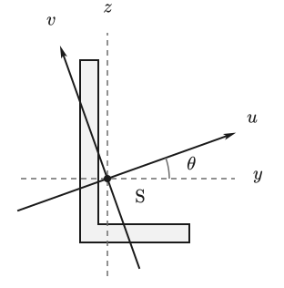
The first principal axis belongs to and has the direction . The angle is measured from to :
The second principal axis is perpendicular to it. If and are equal within the calculation accuracy, every direction is a principal axis; SpanDraft then sets deterministically to zero.
Extreme fibers and section moduli
For the edge stress, the distance of the outermost material points from the bending axis counts. SpanDraft determines it by projecting the contour onto the normal direction of the axis. For a contour point with the centroid coordinates and , the following holds
For , ; for , . For a principal axis, is the direction of the respective other principal axis. The extrema of the projection yield the two extreme fiber distances:
The actual contour is evaluated. For circular arcs, the endpoints are not sufficient: if the extremum of the projection lies within an arc, this point is also taken into account.
The two elastic section moduli of the axis follow from these distances1:
For the T-section, the centroid does not lie at half height. and and thus also and therefore differ (Figure 3).
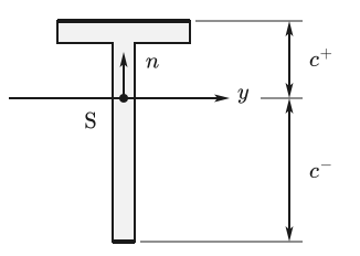
The signs + and − denote geometric sides of the axis: + lies on the side to which points. They are not an automatic assignment to tension or compression. Which side is in tension and which in compression depends on the sign of the bending moment.
Bending axes in SpanDraft
Which axes are available depends on the shape:
- Rectangle, rectangular hollow section, circle, circular hollow section, I/H, U and T section use and . The designation does not depend on which of the two second moments of area is larger: remains the horizontal centroidal axis, even if predominates.
- Circle and circular hollow section are rotationally symmetric and have the same about every centroidal diameter. SpanDraft nevertheless unambiguously uses and .
- The angle section uses its principal axes: with and with .
For the beam model, exactly one of these axes is selected. Its enters the flexural rigidity , as described in the chapter Euler–Bernoulli beam theory. SpanDraft does not perform simultaneous biaxial bending analysis.
and of the selected axis are used later for the elastic stress assessment. The side with the smaller section modulus governs there:
The complete assessment is described in the chapter Bending stress and extreme fibers.
How to select a cross-section and its bending axis is explained in the help under Beam, material and cross-section.
Model limits
The properties cover uniaxial elastic bending. Not included are:
- plastic cross-section reserves: is exclusively the elastic section modulus
- torsion constants
- the shear center
- warping constants
- a spatially coupled or biaxial beam calculation
Entered fillets, in contrast, are not a display detail: they actually enter area, centroid, second moments of area and section moduli as circular arcs.
Rectangle and circle are well-known analytical check cases of this general calculation path. How all eight parametric shapes generate their contours is described in the chapter Parametric cross-section shapes.
Sources
- Dietmar Gross; Werner Hauger; Jörg Schröder; Wolfgang A. Wall. Technische Mechanik 2 — Elastostatik. 15th edition. Springer Vieweg, Berlin, Heidelberg. 2024. DOI 10.1007/978-3-662-68423-8. Accessed .