 SpanDraft
Calculation model and assumptions
From component to beam model
In the beam model, an elongated component is idealized by its beam axis. Instead of describing the complete three-dimensional state of stress and deformation in the volume, the beam model considers the essential motions and internal forces and moments along the axis .1
In SpanDraft, the beam axis begins at the left end of the beam at and runs to the right. The axial displacement describes a motion along this axis. The transverse displacement describes the motion within the bending plane under consideration. In addition, describes the rotation of the cross-section.
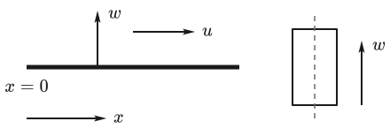
A spatial component can in principle be bent in several planes. The model considers only one planar bending plane at a time. The bending axis of the cross-section selected for it determines, among other things, the second moment of area that is used.1 The positive transverse direction belongs to this bending plane and is not generally identical to the geometric direction of the cross-section.
Material, cross-section and stiffness
For a linear-elastic material, normal stress and strain are proportional1:
Young’s modulus describes the elastic stiffness of the material. The material stiffness alone, however, does not determine the behavior of the beam. The cross-section geometry also influences how strongly the beam deforms under load.
For axial loading, the axial stiffness is decisive. Here denotes the cross-sectional area. For a beam with constant and , the following relation holds between axial displacement and axial force1:
For bending, in contrast, the flexural rigidity is decisive. The second moment of area refers to the bending axis under consideration. A larger leads to a smaller curvature of the beam for the same bending moment.1
The material properties are covered in the chapter Material properties. Cross-sectional area, second moments of area and bending axes are described in the chapter Cross-section geometry and properties.
Implementation in SpanDraft
For a beam, SpanDraft uses a constant material and a constant cross-section. Thus , and the used for the selected bending axis are constant along the entire beam length. The solver uses the flexural rigidity from these; the area is used for self-weight and engineering evaluation.
SpanDraft currently supports no axial loads. The longitudinal direction is therefore not solved as a loaded system: the axial displacement and the axial force are exactly zero everywhere, and an axial support reaction, where present, is likewise zero. In the longitudinal direction, the only check is whether a support prevents the axial rigid-body motion. The remainder of the technical documentation therefore focuses on transverse beam bending.
Linear calculation model
The calculation is materially and geometrically linear.
The material is assumed to be linear-elastic in the range under consideration. After unloading, no plastic deformation remains within this model.1
At the same time, displacements and rotations are assumed to be small. Equilibrium can therefore be formulated on the undeformed system. Changes in the beam geometry caused by the loading do not feed back into stiffness or equilibrium.1
Linearity gives rise to the principle of superposition: the effect of several loads equals the sum of their individual effects.1
Here stands generally for the response of the linear system, for example a displacement, a support reaction or an internal force or moment. Several loads acting at the same time can therefore be superposed. Where distributed loads overlap, their intensities are added with their signs in the common region.1
The principle of superposition holds only within the assumptions of the linear model. Large deformations, plastic material behavior and other nonlinear effects are not included in it.
Euler–Bernoulli assumption
For bending, SpanDraft uses Euler–Bernoulli beam theory. The central kinematic assumption is:
Cross-sections that are plane and perpendicular to the beam axis before deformation remain plane and perpendicular to the deformed beam axis during deformation.1,2
The rotation of a cross-section thus corresponds to the local slope of the beam axis. An additional deformation due to transverse shear is not taken into account in the Euler–Bernoulli model.2,3
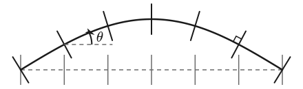
From this assumption follow the relations between deflection, rotation, curvature and bending moment. They are derived in the chapter Euler–Bernoulli beam theory.
Validity and limits
The beam model is a deliberate idealization. Its results hold within the assumptions on which it is based.
Analytical
Linear Euler–Bernoulli theory assumes linear-elastic material behavior as well as small displacements and rotations. Transverse shear deformations and geometric nonlinearity are neglected. Extended beam models can additionally take into account, for example, variable stiffnesses or shear deformations.1,2,3
SpanDraft
SpanDraft calculates a single straight beam with constant material and constant cross-section. Exactly one bending axis, and thus one planar bending plane, is considered per calculation. Spatial beam orientation, simultaneous biaxial bending, a loaded longitudinal direction, elastic supports, support movements, hinges, variable stiffness, non-constant distributed loads, Timoshenko shear deformation, geometric nonlinearity and stability checks such as buckling are not part of the solver.
The excluded effects are not generally negligible in real components. Rather, the model limits define which mechanical problem SpanDraft calculates and under which conditions the results hold.
Further chapters
The help gives a compact overview of the model limits for the application under What SpanDraft calculates – and what it does not.
Euler–Bernoulli beam theory describes the relationship between distributed load, shear force, bending moment, curvature, rotation and deflection.
Loads, supports and internal forces and moments defines the signs used and explains external loads, support reactions, boundary conditions and internal forces and moments.
The later chapters on materials and cross-sections describe the properties from which, among other things, results. How SpanDraft solves the continuous mechanical problem is then covered in the chapter State variables and transfer.
Sources
- Dietmar Gross; Werner Hauger; Jörg Schröder; Wolfgang A. Wall. Technische Mechanik 2 — Elastostatik. 15th edition. Springer Vieweg, Berlin, Heidelberg. 2024. DOI 10.1007/978-3-662-68423-8. Accessed .
- Tomasz Wierzbicki. Euler-Bernoulli Hypothesis. Structural Mechanics, Massachusetts Institute of Technology / MIT OpenCourseWare via Engineering LibreTexts. Accessed .
- COMSOL AB. Beam. Structural Mechanics Module Documentation. Accessed .