 SpanDraft
Physical and metamorphic checks
This chapter belongs to the detailed evidence of the Solver verification. It describes the checks that need no reference solution and therefore apply to all 18 cases.
Principle
A reference comparison needs a known correct value. For cases V07 to V15, the validation catalog stores no analytical reference; there, the reference values come only from the two external programs. Mechanics, however, prescribes relations that every correct solution must satisfy, within one run and between several runs. This gives two kinds of checks:
- Physical checks evaluate a single calculation run.
- Metamorphic checks link several runs. A metamorphic relation is a necessary property of a method across several inputs and their outputs. It does not require known expected values.1
A relation that is satisfied does not prove the solution, because it is only a necessary condition.1 These checks therefore complement the reference comparisons and do not replace them. Both kinds of checks evaluate only the results of the solver and use neither its matrices nor its internal derivatives. Except for the equilibrium check of the reference solutions, which adopts their comparison tolerances, their tolerances are stricter than those of the reference comparisons:
| Quantity | absTol | relTol |
|---|---|---|
| Forces, moments | or Nm | |
| , , | or rad | |
Equilibrium
Global equilibrium is evaluated directly from the inputs and the support reactions calculated by SpanDraft. The resultant of a distributed load from to is , its lever arm .
This gives three comparisons per case. The same equations are applied to the 45 stored references: the check thus also covers the references themselves, except for horizontal equilibrium for PyCBA, which does not supply .
Jump and continuity conditions
At an interior location with a point force, point moment or support, the fields must jump by the external load. This is the local equilibrium relation derived in the chapter Loads, supports and internal forces and moments.
A downward force and a counterclockwise moment thus lower the respective field.
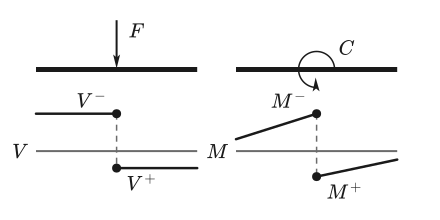
Deflection and rotation, in contrast, must not jump. At every interior location, and hold.
Differential relations
Between the jump locations, the fields are linked through and , here in the SpanDraft sign convention.2 The check computes the derivatives independently using central differences on the output values. It thus remains independent of the internal polynomials of the solver.
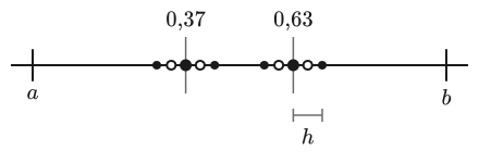
Check locations lie at 37 % and 63 % of each subinterval, the step sizes are and with the interval length . No stencil point crosses a jump location. For a constant distributed load, is quadratic and linear. For these polynomials, the central difference has no truncation error, so the strict tolerance can apply. The second step size checks the numerical stability.
Zero curves in the longitudinal direction
SpanDraft has no axial loads, and all cases therefore contain and . Both are checked as a zero curve at all evaluation points. A loaded axial calculation path is thus not accepted independently.
| Check | Individual comparisons |
|---|---|
| Equilibrium of SpanDraft | 54 |
| Equilibrium of the references | 117 |
| Jumps of and | 56 |
| Continuity of and | 56 |
| Differential relations | 368 |
| Zero curves of and | 512 |
| Total | 1163 |
Scaling and sign reversal
The beam model is linear. For constant and rigid supports, the internal forces and moments are independent of the stiffness, and the deformation is proportional to load and compliance.3 Relations between two calculation runs follow from this. For this purpose, SpanDraft recalculates the transformed input completely.
| Transformation | Reactions, , , | , |
|---|---|---|
| all loads · 2 | doubled | doubled |
| all loads · (−1) | reversed | reversed |
| · 2 | unchanged | halved |
| · 2 | unchanged | halved |
| force of zero at 41 % of the longest subinterval | unchanged | unchanged |
The fields are compared at all evaluation points, not only at the extreme values marked in Figure 3.
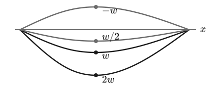
The last row checks that additional event stations do not change the solution. A force of magnitude zero changes nothing about the loading but creates an additional event station with its own nodal result. The check ensures that this station is created and all results remain the same. This follows from the transfer with load integrals: load positions create no unknowns.
Superposition
In the linear model, the solution for a sum of loads is the sum of the individual solutions. Six tests check this in two forms: they split existing load combinations or add a further load.
| Case | Load group 1 | Load group 2 |
|---|---|---|
| V04 | distributed load of the case | additionally −150 N at 0.41 |
| V08 | point force | distributed load |
| V09 | point force of the case | additionally −100 N/m from 0 to 3 m |
| V11 | point forces | distributed load |
| V13 | first distributed load | second distributed load |
| V15 | point force and point moment | distributed load |
Figure 4 shows this for V13: the moment curve of the combination is at every location the sum of the moment curves and of the two distributed loads.
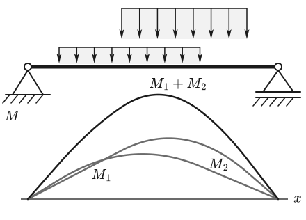
The support reactions and all six fields at the evaluation points of the case are compared.
| Check | Tests | Individual comparisons |
|---|---|---|
| Loads · 2 | 18 | 1599 |
| Loads · (−1) | 18 | 1599 |
| · 2 | 18 | 1599 |
| · 2 | 18 | 1599 |
| Additional event station | 18 | 1599 |
| Superposition | 6 | 838 |
| Total | 96 | 8833 |
Comparison counts per case
The numbers come from the acceptance runs of October 3, 2026 and November 11, 2026, which agree. Cases with a stored analytical reference have three more comparisons in the reference equilibrium, because this reference is added there as an additional reference provider.
| Case | Equilibrium | Field checks | Reference equilibrium | Metamorphic tests | Metamorphic comparisons |
|---|---|---|---|---|---|
| V01 | 3 | 44 | 8 | 5 | 375 |
| V02 | 3 | 24 | 8 | 5 | 255 |
| V03 | 3 | 24 | 8 | 5 | 255 |
| V04 | 3 | 24 | 8 | 6 | 306 |
| V05 | 3 | 44 | 8 | 5 | 375 |
| V06 | 3 | 44 | 8 | 5 | 375 |
| V07 | 3 | 44 | 5 | 5 | 375 |
| V08 | 3 | 104 | 5 | 6 | 882 |
| V09 | 3 | 64 | 5 | 6 | 600 |
| V10 | 3 | 44 | 5 | 5 | 380 |
| V11 | 3 | 124 | 5 | 6 | 1038 |
| V12 | 3 | 24 | 5 | 5 | 270 |
| V13 | 3 | 104 | 5 | 6 | 882 |
| V14 | 3 | 44 | 5 | 5 | 380 |
| V15 | 3 | 164 | 5 | 6 | 1320 |
| V04-S01 | 3 | 24 | 8 | 5 | 255 |
| V04-S02 | 3 | 24 | 8 | 5 | 255 |
| V04-S03 | 3 | 24 | 8 | 5 | 255 |
| Total | 54 | 992 | 117 | 96 | 8833 |
Sources
- Tsong Yueh Chen; Fei-Ching Kuo; Huai Liu; Pak-Lok Poon; Dave Towey; T. H. Tse; Zhi Quan Zhou. Metamorphic Testing: A Review of Challenges and Opportunities. ACM Computing Surveys 51 (1), Article 4. 2018. DOI 10.1145/3143561. Accessed .
- René Alderliesten. Relation Among Distributed Load, Shearing Force, and Bending Moment. Introduction to Aerospace Structures and Materials, Delft University of Technology / TU Delft Open via Engineering LibreTexts. Accessed .
- Jesse Bonanno. IndeterminateBeam: A Python package for solving 1D indeterminate beams. Journal of Open Source Education 4 (40), 111. 2021. DOI 10.21105/jose.00111. Accessed .