 SpanDraft
Continuous results and extreme values
From states to curves
The chapter Stations and equation system provides the states at the mechanical stations. Often, however, a location in between is of interest: the largest deflection of a beam generally lies neither at a support nor under a load.
For each location , SpanDraft first determines the section in which it lies and then evaluates the transfer relations from the start of the section up to , including all loads in between. The calculation always starts directly from the start of the section, not from piece to piece. There is no second solver, no artificial intermediate points and no sampling resolution.
The event stations divide each section into pieces. Within a piece, the load situation does not change, and each quantity there is a single polynomial in the local coordinate. SpanDraft needs these piece polynomials for the search for extreme values.
Analytical
In methods with shape functions, the curve between the nodes is recovered from an approximation. If the true curve does not lie within the approximation, for example a quartic deflection curve under distributed load in a cubic approximation, the interior of the element deviates, and the bending moment there becomes linear instead of quadratic.1
SpanDraft
The transfer relations are the exact solution of the beam equation in the section. The curve between the stations is therefore not an approximation but the same function from which the station values also come. Under a distributed load, the bending moment is quadratic and the shear force linear, as beam theory requires.
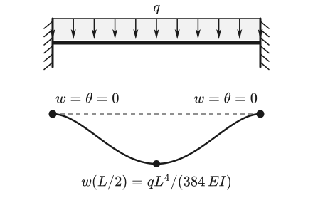
An illustrative example is the beam between two fixed supports under a continuous distributed load. At both mechanical stations, and are prescribed as zero. Only moment and shear force to the right of the left fixed support are unknown; the conditions at the right fixed support determine them as and . The transfer to midspan yields the known value of beam theory.2
Internal forces and moments by differentiation
All quantities of a piece belong to the same function. The relations from Euler–Bernoulli beam theory apply, here in the local coordinate:
The longitudinal part is simpler: without external axial loads, the axial displacement and the axial force are exactly zero at every location and on both sides.
The polynomial degree of each quantity determines its shape in the diagram and the effort for the search for extreme values.
| Quantity | Degree in the piece | At an interior event station |
|---|---|---|
| Deflection | 4 at most | continuous |
| Rotation | 3 at most | continuous |
| Bending moment | 2 at most | jumps at a point moment or reaction moment |
| Shear force | 1 at most | jumps at a point force or support force |
| Displacement | – | zero everywhere without external axial loads |
| Axial force | – | zero everywhere without external axial loads |
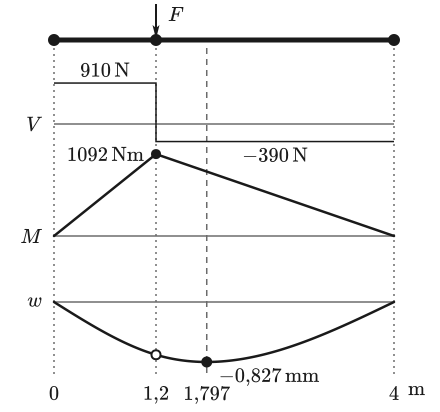
For the example beam, Figure 2 shows the interplay: is piecewise constant and jumps under the force, is linear with a kink, and is piecewise cubic with a continuous tangent. The minimum of does not coincide with any station.
Jump locations and one-sided values
At an interior event station, two pieces with their own polynomials meet. If the station carries a concentrated load or a support reaction, their boundary values for or do not match: the internal force or moment jumps, as derived in the chapter Loads, supports and internal forces and moments.3
At such a location, there is therefore not the one value of the internal force or moment but two one-sided limits. SpanDraft treats them as separate results:
- The left limit is the value of the left piece at the end of the piece, the right limit that of the right piece at the start of the piece. There is no averaging and no smoothing.
- The deformation quantities and are equal on both sides at a station and agree with the output nodal result. Values prescribed at supports are exactly zero on both sides.
- At the beam ends, there is only the value from the beam side: at from the right, at from the left.
- Within a piece, both sides agree, and each position is assigned exactly. A position just next to a station is not rounded to it.
- The start or end of a distributed load produces no jump in or but only changes their slope.
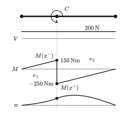
An example: a simply supported beam with carries the moment at . The shear force is +200 N over the entire length. The bending moment, in contrast, jumps from to , that is, by −400 Nm and thus opposite to the applied moment. The deflection remains continuous and smooth.
Global extreme values
For design and assessment, the largest values count. Because , and are polynomials in each piece, SpanDraft does not have to search for their extreme values on a grid. The piece boundaries and the zeros of the respective derivative suffice as candidates: for and for .
| Quantity | Candidates per piece |
|---|---|
| Deflection | both piece ends and all interior zeros of |
| Bending moment | both one-sided piece end values and the interior zero of |
| Shear force | both one-sided piece end values, because is linear in the piece |
From all candidates of a beam, SpanDraft selects the signed minimum and maximum, each with position and, if needed, side. This already happens during solving and thus does not depend on how the result is displayed later.
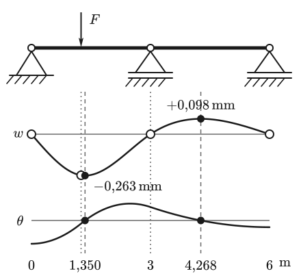
Figure 4 shows the candidates on a continuous beam. The minimum of lies there only 10 cm from the force location.
That this is worthwhile is shown by the example beam. A grid of 0.5 m would hit neither the force location nor the minimum:
| Quantity | Analytical | SpanDraft | Grid 0.5 m |
|---|---|---|---|
| Minimum of in mm | −0.827359 | −0.827359 | −0.817143 |
| Location of the minimum in m | 1.79697 | 1.79697 | 2.0 |
| Maximum of in Nm | 1092.00 | 1092.00 | 975.000 |
| Location of the maximum in m | 1.2 | 1.2 | 1.5 |
The analytical values follow, for a force in the left half of the beam and with , from , and .2 The grid values were evaluated with SpanDraft at the grid points: they lie on the correct function but miss the bending moment by about 11 %.
Each minimum and maximum is stated with exactly one representative location. If several locations have the same value, the smallest position counts and, for equal position, the left side. A constant section is represented by an endpoint, not as an interval. The diagram can therefore show an equally large value at another location without a second extremum being marked there.
Deep dive: root finding and rounding limits
The zeros are determined without sample points. The polynomial is first scaled by its largest coefficient; vanishing leading coefficients reduce the degree. Linear polynomials are solved directly. For quadratic polynomials of the form , SpanDraft uses the cancellation-resistant form of the solution formula, which does not subtract two almost equal numbers from each other.4
Here copysign(x, b) takes the sign of for the magnitude . Unlike an ordinary signum function, this operation also returns a defined sign for . As a result, does not become zero for a positive discriminant merely because .
Cubic polynomials, such as under a distributed load, SpanDraft splits into monotonic intervals using the real zeros of their derivative. In each interval whose ends show a sign change, it searches for the zero by bisection with at most 128 steps. The stationary points themselves are checked separately for multiple roots, because the sign change is missing there. The bisection ends according to the interval width, not according to a blanket threshold for a small function value. SpanDraft evaluates the polynomial itself in the coordinate between 0 and 1, normalized to the piece length, using the Horner scheme.4
The rounding rules apply only within this polynomial calculation and are based on . Zeros that are at most away from 0 or 1 are assigned to the respective boundary, whether they lie inside or outside the interval. Those lying further outside are discarded, and zeros at a distance of up to are merged. If the discriminant lies within its rounding uncertainty of around zero, the zero counts as double with . For ties in values, a relative comparison of without an absolute threshold applies, because such a threshold would conceal real differences in very small load cases. The exact position comparisons in the model remain unaffected.
Diagram and calculation
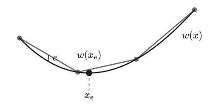
A result diagram visualizes the calculation but is a separate downstream step. It reads out the finished functions and connects points on them by straight lines. The mechanics is complete at this point. Between two points, the chord deviates from the function by the distance (Figure 5). This deviation arises only in the drawing. In the SpanDraft diagram, the analytical extremum additionally always lies on a point of its own.
| Feature | Continuous calculation | Diagram |
|---|---|---|
| Content | piecewise analytical functions | polyline of points on these functions |
| Resolution | none, every location can be evaluated | depends on the screen |
| Extreme values | from piece ends and zeros | takes value and location from the calculation |
| Jumps | two one-sided values | vertical connection of both values |
| Influence of window size | none | different points, same function |
SpanDraft refines the polyline adaptively: points in are at most 8 screen pixels apart, and the chord is to deviate from the function by at most half a pixel at the checked intermediate locations. Event stations and the locations of the extreme values are fixed points of the polyline. Each piece between two event stations is sampled separately, so that a line never interpolates across a jump.
For reading values, this means: the extreme value markers come from the calculation, not from the polyline. A vertical line in the diagram is the connection of two one-sided values and not a curve with infinite slope. Anyone stating a value at a jump location must therefore also name the side.
Where the application displays diagrams, extreme value markers and support reactions is explained in the help under Result diagrams and support reactions.
How reliable the results are
Within the model, the functions are analytical, but the calculation itself runs in floating-point numbers. SpanDraft outputs a value only if its error relative to the exact solution of the model is demonstrably below a fixed bound; the chapter Numerical solution and accuracy describes this criterion. For curves and extreme values, this means:
- Prescribed values such as at a support or at a free end are exactly zero. Transferred values that vanish only in theory, in contrast, can show small rounding residues; they are not blanket-set to zero.
- The error bound applies to the value at the output location and side. It says nothing about how accurately the location of an extreme value is determined.
- Closely adjacent or multiple zeros are harder to determine in their position than simple ones. Below the rounding resolution of the coefficients, they are not reported separately. In such cases, the location of an extreme value reacts more sensitively than its value, because the function runs flat there.
- Every output extreme value can be reproduced at its location and side as an ordinary field value.
The fields and extreme values are checked against independent references, including jump locations, derivative relations and extreme locations between the stations. The chapter Solver verification documents this evidence.
All statements of this chapter apply to the Euler–Bernoulli model. The solver does not assess strength: elastic bending stress and the ratio to the strength value are a separate evaluation, described in the chapters Bending stress and extreme fibers and Safety factor and assessment limits.
Sources
- Carlos A. Felippa. Variational Formulation of Plane Beam Element. Introduction to Finite Element Methods, Chapter 12, University of Colorado Boulder. Accessed .
- Dietmar Gross; Werner Hauger; Jörg Schröder; Wolfgang A. Wall. Technische Mechanik 2 — Elastostatik. 15th edition. Springer Vieweg, Berlin, Heidelberg. 2024. DOI 10.1007/978-3-662-68423-8. Accessed .
- René Alderliesten. Relation Among Distributed Load, Shearing Force, and Bending Moment. Introduction to Aerospace Structures and Materials, Delft University of Technology / TU Delft Open via Engineering LibreTexts. Accessed .
- Nicholas J. Higham. Accuracy and Stability of Numerical Algorithms. 2nd edition. Society for Industrial and Applied Mathematics, Philadelphia. 2002. DOI 10.1137/1.9780898718027. Accessed .