 SpanDraft
State variables and transfer
From boundary value problem to transfer
Euler–Bernoulli beam theory describes bending with four first-order differential relations. In the SpanDraft signs, they read:
Combined, they yield . Supports and beam ends prescribe boundary conditions at different locations; mathematically, this is a boundary value problem. By hand, it is integrated section by section: each section brings four constants of integration, which are determined from boundary and transition conditions.
SpanDraft uses the same integration but arranges it differently. The four constants of integration of a section are nothing other than the four quantities at the start of the section. They form the state
If the state at one location is known, equation (1) fixes it in the entire section, as long as there are no supports there. In engineering mechanics, this procedure is called the transfer matrix method; in numerics, for several coupled sections, the method is called multiple shooting.1,2 How the sections are assembled at supports and beam ends is described in the chapter Stations and equation system.
Analytical
In hand calculation, the constants of integration of each section are carried as unknown numbers. For each support and load case, a separate equation system arises from boundary and transition conditions.
SpanDraft
SpanDraft carries the same constants as physical state variables at the start of the section. The transfer within the section is the same for all models; only the conditions at supports and ends differ.
Transfer relations within the section
A section begins at a station and extends to the next one. The local coordinate is measured from the start of the section. The free-body cut of a piece from the station to the location shows what the state at this location is composed of: the state at the start and the loads in between.
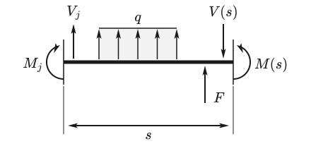
Equilibrium of the vertical forces yields , moment equilibrium about the right cut face yields . Integrating twice yields rotation and deflection. With constant in the section, the following holds:
Here is the state immediately to the right of the station. The load integrals , , and contain all loads behind the station up to the location . Loads exactly at the station are already contained in the state to the right of it. A load exactly at the location is included in the right-hand limit but not in the left-hand limit. Without a load, the load integrals are zero.
The structure becomes clear in matrix form. The state at the location is the transferred initial state plus the load contribution:
The transfer matrix is an upper triangular matrix with ones on the main diagonal. Its entries are polynomials in s; exponential functions, as occur for example with elastic foundations, do not appear. For a very short section, it is nearly the identity matrix: the states at its two ends differ only slightly, and large numbers do not arise. The numerical solution makes use of this property.
Load integrals
The load integrals describe how a load changes the state behind its point of application. A load at the location acts only from onward. This is expressed by the Macaulay bracket (also called Föppl bracket):3
For , the bracket is continuous and zero at the location . For , it jumps there from 0 to 1. At the jump location itself, it is evaluated not as a function value but as a one-sided limit, corresponding to the side that SpanDraft explicitly requires for every evaluation: on the left () with 0, on the right () with 1. The left-hand state at a point force or a point moment thus does not yet contain the load, the right-hand state already contains it completely.
For the three load types of SpanDraft, the load integrals follow from equation (1) by integration. The point force makes jump, the point moment makes jump by −, and the distributed load between and changes the slope of . The signs follow the chapter Loads, supports and internal forces and moments: forces and distributed loads are positive upward, moments counterclockwise.
| Load | ||
|---|---|---|
| Point force at | ||
| Point moment at | 0 | |
| Distributed load from to |
Several loads are added. The contributions for rotation and deflection arise by further integration, with each term integrated by the same rule; they are divided by only in equation (3):
For the distributed load, this yields, for example,
Figure 2 shows the shear force contribution of a distributed load: it grows linearly in the loaded region and remains constant behind it, equal to the resultant.
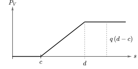
The loads thus act exactly at their entered position and over their exact limits. A distributed load is not replaced by point loads and not distributed onto neighboring points. A load changes only the load contribution in equation (4), not the transfer matrix.
Deep dive: cancellation-resistant evaluation of short loads
For a location behind a distributed load with length and distance from the end of the load, the load integrals contain differences such as . For a very short load far in front of the location, both terms are almost equal in size, and their difference loses digits in floating-point arithmetic. SpanDraft therefore evaluates the integrals in an expanded form in which only positive terms in and appear:4
The form shows the mechanics directly: behind the load, its resultant acts with the lever arm to the middle of the load. Even a load only nanometers long thus retains its resultant and its first moment. SpanDraft always forms distances directly from the stored coordinates, never from already rounded intermediate values.
Example: cantilever under distributed load
A cantilever fixed at the left with carries the distributed load over its entire length; . The beam consists of a single section. At the fixed support, and ; the unknowns are and . At the free end, moment and shear force must vanish. With equation (3) and the load integrals of the distributed load, it follows:
This is the well-known solution of beam theory.3 With the numbers, , and result. SpanDraft delivers the same values: the support reactions are 1500 N and 2250 Nm, the end displacement −3.01339 mm. No discretization or mesh refinement is required.
Several distributed loads and self-weight
Overlapping distributed loads remain separate loads. Their load integrals are added; at each load boundary, the resulting intensity changes, and in between it is constant. The load boundaries are locations at which the curve changes, but not locations at which new unknowns arise. SpanDraft calls them event stations.
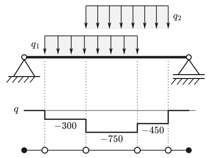
The self-weight also takes the same path: it is derived in the model as a constant distributed load over the entire length and needs no special treatment.
Why there is no discretization error
For the load types of SpanDraft, the load integrals are polynomials, and the transfer relations (3) are the exact solution of equation (1) in the section. Between two stations, nothing is approximated. Two properties follow from this:
- The curve is piecewise polynomial: for constant distributed loads, is of degree four at most, of degree three, of degree two and of degree one.
- Additional evaluation locations or loads of magnitude zero change nothing in the results. A test run with the single-span beam from the chapter Stations and equation system and 38 additional point forces of magnitude zero yields the same minimum of the deflection down to the last bit.
Exact means only this here: the result reproduces the model equation. The calculation itself runs in floating-point numbers; how accurate it is and when SpanDraft withholds a result is described in the chapter Numerical solution and accuracy. Whether the model fits the component is a different question, which the chapter Calculation model and assumptions covers.
Limits of the formulation
The closed-form transfer depends on the assumptions of the model:
- is constant over the entire length. Variable cross-sections are not supported.
- Distributed loads are constant. Linearly or otherwise varying line loads do not exist.
- Shear deformation is absent because the beam follows Euler–Bernoulli kinematics.
- Equilibrium is formulated on the undeformed beam. Geometric nonlinearity is not captured.
- There are no external axial loads. The longitudinal direction therefore needs no transfer of its own: and are zero everywhere.
Sources
- Eduard C. Pestel; Frederick A. Leckie. Matrix Methods in Elastomechanics. McGraw-Hill, New York. 1963. Accessed .
- Uri M. Ascher; Robert M. M. Mattheij; Robert D. Russell. Numerical Solution of Boundary Value Problems for Ordinary Differential Equations. Classics in Applied Mathematics 13. Society for Industrial and Applied Mathematics, Philadelphia. 1995. DOI 10.1137/1.9781611971231. Accessed .
- Dietmar Gross; Werner Hauger; Jörg Schröder; Wolfgang A. Wall. Technische Mechanik 2 — Elastostatik. 15th edition. Springer Vieweg, Berlin, Heidelberg. 2024. DOI 10.1007/978-3-662-68423-8. Accessed .
- Nicholas J. Higham. Accuracy and Stability of Numerical Algorithms. 2nd edition. Society for Industrial and Applied Mathematics, Philadelphia. 2002. DOI 10.1137/1.9780898718027. Accessed .